
Simple robust optimization tutorial
Published:
Let’s say that you are working in a local taxi company where they want to develop their in-house navigation software. This navigation software is responsible for showing the taxi drivers the optimum directions to the destination or pick-up points. Naturally, arriving quickly is crucial—after all, as the saying goes, time is money!
It sounds straightforward, right? As the engineer or scientist in the team, you might directly frame the problem as the shortest path problem. A logical approach would be to solve it using linear programming or Dijkstra’s algorithm to determine the optimal route. But wait, have you considered that your company operates in a bustling metropolitan city? Traffic jams, roadblocks, and unexpected delays can happen anytime, anywhere. The route is full of uncertainties! So, how do you tackle this problem?
There are several ways to model uncertainty, and a probabilistic approach might seem like the natural choice. However, since your team is relatively new and lacks the resources to collect enough traffic data for accurate probability distributions, this approach isn’t feasible—at least for now. So instead, you can choose an interval set! An interval set is defined by the lower and upper bound of a possible value:
\[t_{\dagger} = [\underline{t},\overline{t}].\]This allows you to represent travel time on each road segment (graph edge) as an interval rather than a fixed value, accounting for possible variations.
To make this more concrete, let’s consider a simple routing problem using the following graph (download here). Throughout this tutorial, we’ll use Python and Gurobi (academic license) as our optimisation solver. First, let’s import the required libraries.
import numpy as np
import pandas as pd
import networkx as nx
import matplotlib.pyplot as plt
import gurobipy as gp
Since the data is in text format, we have to parse the data into the graph components:
def parse_data(filename):
    with open(filename) as f:
        lines = [line.rstrip('\n') for line in f]
    k = int(lines[0])  # maximum number of arcs suggested
    nodes = lines[1].split()  # list of nodes
    edges = []  # list of edges
    edge_labels = {}  # edge labels
    for line in lines[2:]:
        splitline = line.split()
        edge = tuple(splitline[:2])
        edges.append(edge)
        edge_labels [edge] = [float(a) for a in splitline[2:]]

    edge_list= ["_".join(tup) for tup in edges]
    return k, nodes, edge_list, edge_labels
And finally, draw the graph:
k, nodes, edge_list, edge_labels = parse_data("simple_route.dat")

G = nx.DiGraph()
edges = edge_labels.keys()
G.add_edges_from(edges)

pos = nx.spring_layout(G, seed=42)
nx.draw(G, pos, with_labels=True)
nx.draw_networkx_edge_labels(
    G, pos,
    edge_labels=edge_labels,
    font_color='red'
)
plt.show()
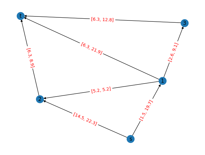
Figure 1. Simple routing problem with uncertain weight.
In this problem, the taxi driver needs to travel from $s$ to $t$ using one of several possible routes, each affected by interval uncertainty. For example, on the path $s \rightarrow 1$, the travel time can range from a minimum of 1.5 minutes to a maximum of 19.7 minutes, depending on factors like traffic congestion or roadblocks. This variability means that the actual time required for each route isn’t fixed but lies within a given interval, adding uncertainty to the decision-making process. From the data, we can also extract the edge labels and infer each possible path. The extracted edge labels are given by:
{('s', '1'): [1.5, 19.7],
 ('s', '2'): [14.5, 22.3],
 ('1', '2'): [5.2, 5.2],
 ('1', 't'): [6.3, 21.9],
 ('1', '3'): [2.6, 9.1],
 ('2', 't'): [6.3, 8.9],
 ('3', 't'): [6.3, 12.8]}
while each possible path can be obtained using nx.all_simple_paths(), resulting in:
[['s', '1', '2', 't'], ['s', '1', 't'], ['s', '1', '3', 't'], ['s', '2', 't']]
It is important to note that in this tutorial, we simplify the problem a little bit. We determine $k=1$, where $k$ is the maximum number of arcs for which the travel time will be at the upper bound, with the travel time of all other arcs being at the lower bound. Simply put, when the algorithms plan the optimal direction, it only assumes that only one road section will be on the maximum value. Thus, we can extract the uncertainty set which corresponds to this setting:
def uncset(edge_labels):
  # Note: This function is not generalizable to k>1
  uset = []
  for i in range(len(edge_labels)):
      temp = []
      for j,val in enumerate(edge_labels.values()):
          if i == j:
              temp.append(val[1])
          else:
              temp.append(val[0])
      uset.append(temp)

  return uset
which obtains the following uncertainty set:
[[19.7, 14.5, 5.2, 6.3, 2.6, 6.3, 6.3],
 [1.5, 22.3, 5.2, 6.3, 2.6, 6.3, 6.3],
 [1.5, 14.5, 5.2, 6.3, 2.6, 6.3, 6.3],
 [1.5, 14.5, 5.2, 21.9, 2.6, 6.3, 6.3],
 [1.5, 14.5, 5.2, 6.3, 9.1, 6.3, 6.3],
 [1.5, 14.5, 5.2, 6.3, 2.6, 8.9, 6.3],
 [1.5, 14.5, 5.2, 6.3, 2.6, 6.3, 12.8]]
where each column in the array corresponds to each arc in the graph.
Robust Optimisation Formulation
There are several strategies to find a robust solution. Depending on the circumstances, we can choose or modify it as we like, tailored to the specific problem. In this article, we will discuss three common strategies: worst-case, additive regret, and multiplicative regret.
Worst-case
As the name implies, this strategy searches for the optimum worst-case solution. In this case, the objective is to minimise the worst-case(maximum) solution. This statement is mathematically translated to:
\[\min_{x \in X} \max_{c \in \mathcal{U}} c(x).\]Since we are optimising (minimising) an uncertain objective, we can rewrite the formulation as:
\[\begin{align} \min \quad & t \\ \text{s.t.} \quad & t \geq c(x), \ \forall c \in \mathcal{U}\\ & \sum_{(s,v)\in\text{Node}} x_{(s,v)} = 1\\ & - \sum_{(v,t)\in\text{Node}} x_{(v,t)} = -1\\ & \sum x_{(v,w)} - \sum x_{(u,v)} = 0, \ \forall v \neq s,t\\ & x \in \{0,1\} \end{align}\]It is important to note that the constraints consist of the constraint from the uncertainty set, the constraint from the source (start) and sink (finish), as well as the flow conservation constraints. Translating the problem into Python code:
# Defining model
m = gp.Model("worstcase")
x = gp.tupledict()

# Define variables
for (v1,v2) in edge_labels.keys():
    x[v1,v2] = m.addVar(vtype="B", name=f"x_{v1}_{v2}", lb=0.0)

t = m.addVar(name="t", lb=0.0)

# Set objective
m.setObjective(t, gp.GRB.MINIMIZE)

# adding flow conservation constraints
for v in G.nodes:
    # we need to skip the source (0) and the sink (7)
    if v not in ['s','t']:
        # we collect the predecessor variables
        expr1 = gp.quicksum(x[i,v] for i in G.predecessors(v))

        # we collect the successor variables
        expr2 = gp.quicksum(x[v, j] for j in G.successors(v))

        # we add the constraint
        m.addLConstr(expr1 - expr2 == 0)

# Adding source and sink constraints
so = gp.quicksum(x['s',i] for i in G.successors('s'))
si = gp.quicksum(x[j,'t'] for j in G.predecessors('t'))
m.addLConstr(so == 1)
m.addLConstr(si == 1)

# Adding constraints from uncertainty set
for u in u_set:
    con = gp.quicksum(x[n1,n2] * u[i] for i,(n1,n2) in enumerate(edge_labels.keys()))
    m.addLConstr(t >= con)

# Run optimizer
m.optimize()
Extracting the result yields:
result = {var.VarName : var.x for var in m.getVars()}
{'x_s_1': 1.0,
 'x_s_2': 0.0,
 'x_1_2': -0.0,
 'x_1_t': 1.0,
 'x_1_3': -0.0,
 'x_2_t': 0.0,
 'x_3_t': 0.0,
 't': 26.0}
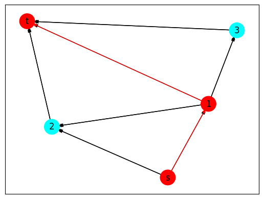
Figure 2. Worst-case optimisation result.
Additive Regret
TO BE CONTINUED…
How to cite this article:
@misc{faza2025robustopttutorial,
   author =       {Faza, Ghifari Adam},
   title =        {Simple robust optimization tutorial},
   month =        {February},
   year =         {2025},
   url =          {https://fazaghifari.github.io/posts/2025/03/rob-opt-en/},
 }