Simple Vector Field Prediction using Proper Orthogonal Decomposition and Polynomial Chaos Expansion (POD-PCE)

In this article, we explore the utilization of proper orthogonal decomposition (POD) and polynomial chaos expansion (PCE) as a surrogate model to forecast flow field behavior at unseen time steps. When compared to other standard surrogate models like standard PCE regression or standard Gaussian process (GP) regression, the integration of POD presents advantages in the analysis of vector-field data, by converting the complete solution of a vector field into a collection of simpler representations that are more manageable.

The Indonesian version of this article can be found here.

Proper orthogonal decomposition (POD), also known as Karhunen-Loéve decomposition [1] is a popular method in engineering analysis to obtain the approximation of lower dimension representation of turbulent flows [2], structural analysis [3], and dynamical system [4]. In simple terms, POD transforms the full solution of a vector field into a set of simpler representations that can be easily handled. For example, we can decompose the fluid flow vector field as shown in image/video below to its simpler representation:

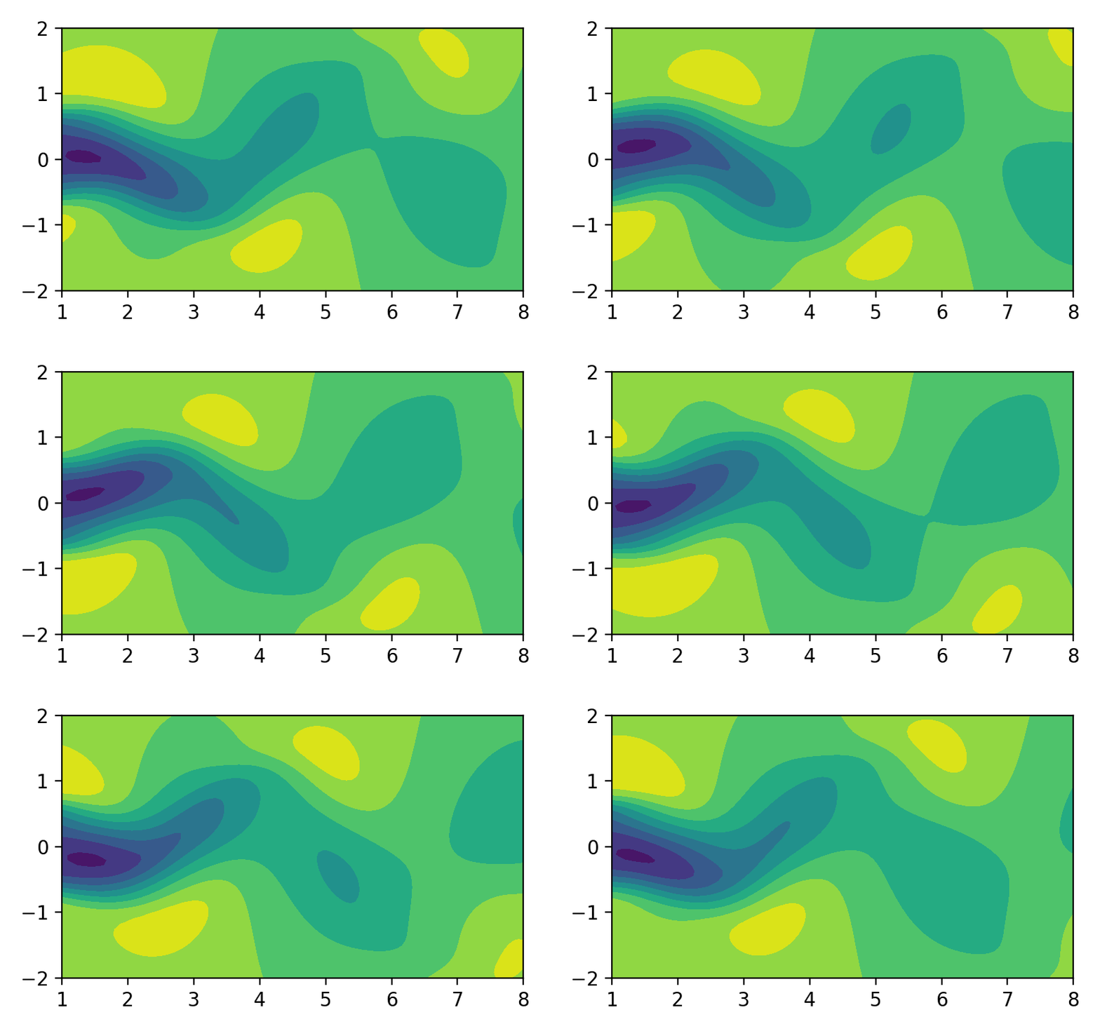
Figure 1. Fluid flow illustration.

If you are unfamiliar with this concept, you might be questioning “Why would I need a simpler/lower dimension representation of the fluid flow?”. One of the most common uses is that we can use the lower dimension representation of the problem to predict the behaviour of the problem/system given unknown parameter(s). For example, if the video above depicts fluid flow from $t=0$ to $t=5$, we can use the lower-dimensional representation to predict the flow’s shape at $t=6$.

Consider that a single vector field can be constructed from a few to millions of elements or discretization points. Predicting each element for every time step is a complex task. Therefore, by employing Proper Orthogonal Decomposition (POD), we simplify the problem by predicting the lower-dimensional representation of the system rather than each individual element.

POD Formulation

Input Data

POD requires an input format in the shape of $N \times m$ where $N$ is the number of elements or discretization in the problem, and $m$ is the number of parameter variations. In the context of our fluid flow scenario, the varying parameter is time $t$. Therefore, if desired, you can replace $m$ with $t$ in our current example. However, for the sake of generalization, I am using $m$. This $N \times m$ matrix is often referred to as the snapshot matrix. The schematic of the snapshot matrix construction is given in Figure 2:

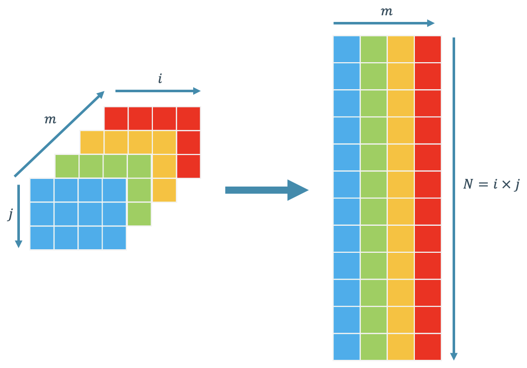
Figure 2. Snapshot matrix construction schematics.

In the context of our fluid flow case, we should flatten the flow field data at each time step as shown in Figure 3. The flattened data are then arranged in a way such that each column of the snapshot matrix represents one timestep.

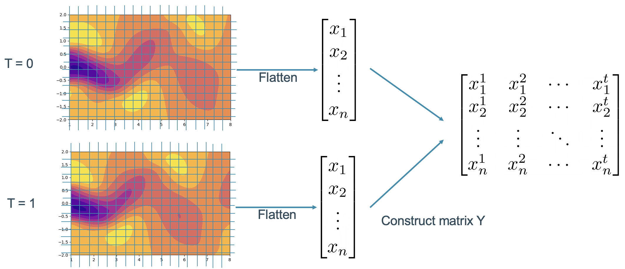
Figure 3. Fluid flow snapshot matrix construction process.

To make things to be more practical, I will provide the Python code as a companion. The dataset that is used in this article can be downloaded here.

The given dataset has several components, namely U_star (x and y velocity field component), p_star (pressure field), t_star (time stamp), and X_star (spatial coordinate). In this article, we will only consider the x velocity component as our variable of interest and the spatial coordinate for plotting. First, we extract the dataset

import numpy as np
import scipy.io
import matplotlib.pyplot as plt

data = scipy.io.loadmat("cylinder_nektar_wake.mat")
u_star = data['U_star']  # N x 2 x T -- 2 indicates u_x (1st axis) and u_y (2nd axis)
p_star = data['p_star']  # N x T
t_star = data['t']  # T x 1
x_star = data['X_star']  # N x 2

Notice that all variables are already flattened. So actually, we don’t need to flatten each variable by ourselves. However, it is important to know that for plotting purposes, we need to reshape the spatial coordinates x_star into the desired shape of $50 \times 100$. Notice that the shape of x_star is $N \times 2$, where the first column corresponds to the $x$ coordinate and the second column corresponds to $y$ coordinate.

# Reshape Data
x_grid = x_star[:,0].reshape(50,100)
y_grid = x_star[:,1].reshape(50,100)

As we have decided that we will only consider the x velocity component as our variable of interest, we will only select the first component of the second axis from u_star u_star[:,0,:]. Notice that by selecting this, we already make an $N \times T$ matrix, which is the intended shape of our snapshot matrix. Therefore:

snapshot = u_star[:,0,:]

Up to this point, we are basically done. However, if you want to plot one realization (one timestep) from the snapshot matrix, you can choose one column from the snapshot matrix, reshape the selected column into $50 \times 100$, and then plot a contour. The plotting result is supposed to look like Figure 4

single_snapshot = snapshot[:,42]  # Select one column (any column, here I choose column 42)
ux_grid = single_snapshot.reshape(50,100)  # Reshape selected column to 50 x 100

# Simple Plotting
plt.contourf(x_grid,y_grid,ux_grid)
plt.xlabel('x')
plt.ylabel('y')

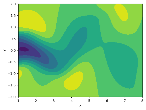
Figure 4. Single timestep fluid flow plot.

Matrix Decomposition

At the core of POD is the singular value decomposition (SVD) technique [5], which you may have encountered in your linear algebra course. For those who may have forgotten their linear algebra lessons or have not studied it, I’ll make sure to explain the concept of POD as clearly and simply as possible.

Supposed that we have any matrix $Y$, we can decompose $Y$ into $U$, $\Sigma$, and $V$ matrices (I will not dive into the details of the matrix decomposition, as nowadays we can use a library such as numpy to perform SVD. However, if you are interested I strongly recommend this video by Prof. Gilbert Strang himself 😉)

In the context of our fluid flow POD, the $Y$ matrix serves as our snapshot matrix. Matrix $U$ can be interpreted as a matrix that represents spatial components. Similarly, matrix $V$ is a matrix that represents the other parameter components, or in this case, the time component. The $\Sigma_r$ matrix is an $r$-rank diagonal matrix that represents the “strength” or the importance of the corresponding basis. The diagonal of $\Sigma_r$ consists of the singular values of $Y$ which are arranged in decreasing order such that $\sigma_1 \geq \sigma_2 \geq \ldots \geq \sigma_r$. The rank $r$ of the Singular Value Decomposition (SVD) is determined by the smallest number between $N$ and $m$, mathematically written as $\min(N,m)$. The corresponding shape after the decomposition process is illustrated in Figure 5.

Figure 5. SVD illustration.

In Python, the SVD decomposition can be done easily. Here, we should pass the parameter full_matrices=False in order to get the desired output shape. Otherwise, we won’t get the desired shape (you can read further (here)[https://numpy.org/doc/stable/reference/generated/numpy.linalg.svd.html]). As explained in the documentation, the default shape of s is a $r \times 1$ array, which mean in order to be consistent with our definition of $\Sigma_r$ we should transform it into a diagonal matrix. You should also pay attention that the output vt is already the transposed version of $V$.

u,s,vt = np.linalg.svd(snapshot,full_matrices=False)
sigma = np.diag(s)

By assuming that $r = \min(N,m)$, you might notice that the final dimension of matrix $U$ is still the same with the original snapshot matrix. The fact that the decomposition result holds the same shape with the original matrix is computationally memory inefficient. Thus, we can further truncate $r$ by choosing a number $k$ such that $k < r$. First, we can set $k$ as a user-defined variable. Or second we can approximate the number of $k$ by:

where $\sigma_i$ is the diagonal element of $\Sigma$ arranged in decreasing order such that $\sigma_1 \geq \sigma_2 \geq \ldots \geq \sigma_r$. Variable $\alpha$ can be interpreted as the amount of “variation” that can be explained by the truncated model. Or, in my free interpretation, it’s the level of “accuracy” that we would like to retain in the truncated model. We typically choose $\alpha = 0.99$. (Note: the code for user-defined k and the corresponding truncation is left to the reader as an exercise.)

# Determine number k
temp = 0
alpha = 0.99
diagsum = np.sum(s)
for idx, sigma in enumerate(s):
    temp += sigma
    ratio = temp/diagsum

    if ratio >= alpha:
        k = idx
        break

# truncate matrices
s_trunc = s[:k]
u_trunc = u[:,:k]
vt_trunc = vt[:k,:]
sigma_trunc = np.diag(s_trunc)

Hence, now we have:

In POD, we often define a POD coefficients $B$, where $B_k = \Sigma_k V^T_k$, $B_k \in \mathbb{R}^{k \times m}$. Thus, our equation now becomes:

pod_coeff = sigma_trunc @ vt_trunc

The Proper Orthogonal Decomposition (POD) comprises two major components: the spatial basis matrix $U$ and the physical parameter component represented by the POD coefficient $B$. The spatial basis matrix $U$, as the name implies, provides a foundation for constructing the full-order solution. Each column in the matrix $U$ represents different modes of the full-order solution. Put simply, these modes serve as the fundamental ingredients (basis) for forming the full-order solution. By blending (adding) these modes with the appropriate proportion (coefficients), we can derive the correct full-order solution. The plot depicting the first-order basis, second-order basis, and full-order solution can be found in Figure 6. At this juncture, our work with matrix $U$ is complete, and we will preserve this matrix for future use.

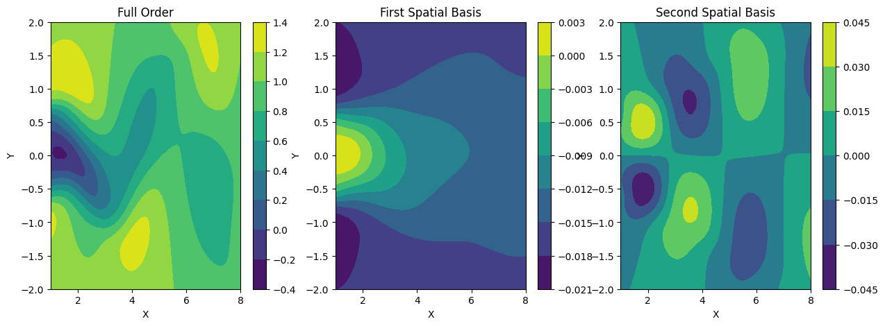
Figure 6. Different spatial basis up to second-order basis.

A single column in the POD coefficient matrix $B$ provides a correct “proportion” for the spatial basis $U$ to form a single full-order solution for a given parameter, or in our case, for one timestep, represented by a single column in our snapshot matrix $Y$. As shown in Figure 7, the red column in $Y$ represents the vector field of the problem for a given parameter. Similarly, each green column in $B$, represents a vector of coefficients for the same parameter as the red column. In other words, if the red column corresponds to the flattened fluid flow at $t=0$, then the green column corresponds to a set of coefficients that govern the spatial basis matrix $U$ at $t=0$ to form the red column.

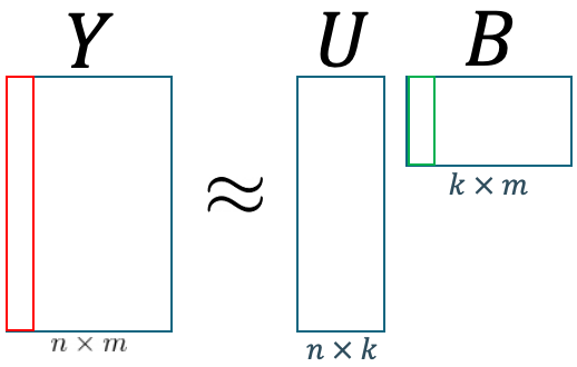
Figure 7. POD illustrations.

By this logic, if we are able to somehow predict the value of coefficients at any $t$, then we are also able to predict the fluid flow behavior at any $y$. This implies that we can also predict the future fluid flow behaviour if we are able to predict the future value of our POD. coefficients.

Regression

General Idea

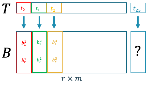
Figure 8. Mapping between problem parameters (time) to POD coefficients.

Figure 8 shows that if we are able to construct a function that maps between the physical parameters and the POD coefficient, then we can predict the POD coefficient given an unseen/unknown value of the parameter. Given that we already have the data, we can construct a regressor that learns from the available data to be able to approximate the POD coefficients given input parameters.

Basically, we can employ any kind of regressor that is able to predict a continuous value. However, we should be aware that most of the regression techniques, at least the ones that are available in scikit-learn, are only able to handle one-to-one or many-to-one mapping. This means that the regression models are able to handle, at most, many inputs and single output. However, in our case, we have a single input and multiple outputs with the size of $k$. Hence, in our case, we need $k$ number of regressor. The first regressor uses the first row of matrix $B$ as its target variable, the second regressor uses the second row of matrix $B$, and so on as illustrated in Figure 9.

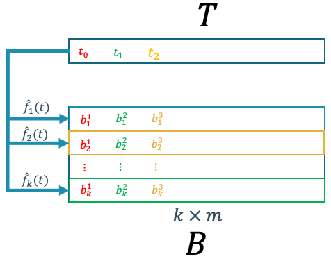
Figure 9. POD coefficient regression scheme.

Polynomial Chaos Expansion (PCE) Regression

PCE regression [6] is a popular technique in the field of uncertainty quantification (UQ), where it is often used as an approximation (surrogate model) of expensive evaluation functions such as experiments and expensive simulations. A simple polynomial regression is mathematically written as:

where $\alpha$ is the degree of the polynomial, and $c_\alpha$ is the coefficient for the corresponding degree. Therefore, if for example, we have $\alpha = 2$, then we have a quadratic formula $\hat{f}(X) = c_0 + c_1 X + c_2 X^2$.

PCE regression has a similar structure as polynomial regression. However, instead of using the original input as a basis, PCE uses an orthogonal polynomial basis in terms of random variable such as Hermite polynomials, Laguerre polynomials, Legendre polynomials, etc (Legendre polynomial illustration given in Figure 10). The orthogonal polynomial basis is written as $\phi(X)$. Thus, we have:

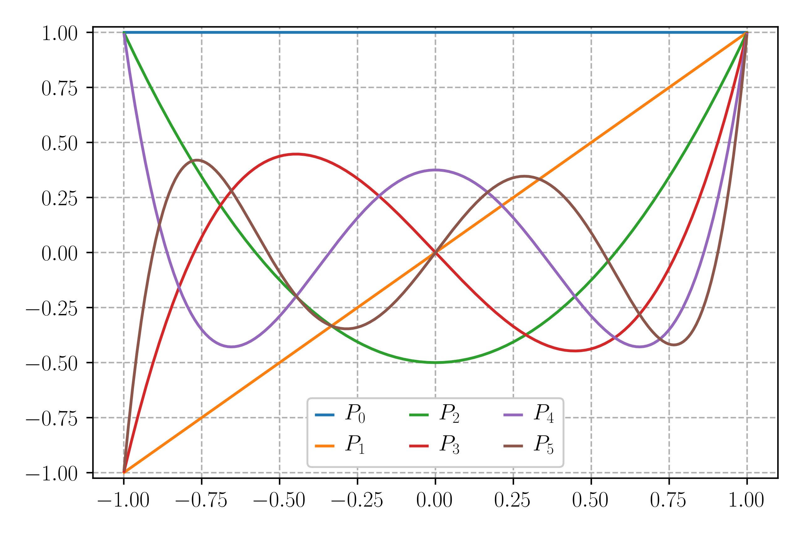
Figure 10. The first six Legendre polynomials [7].

The advantage of using these kinds of orthogonal polynomials instead of the original input as a basis is that it offers more flexibility to fit a more complex relation between the parameter of the physical problem and the POD coefficients.

To avoid the high computational effort in equation 6 due to the summation over the whole domain, we replace the infinite summation in an infinite domain with a finite-term summation:

where the number of expansion terms $S+1$ is a function of the dimensions $(d)$ of $\boldsymbol{X}$ and the highest order $(p)$ of the polynomials $\phi(X)$ [8], defined as:

Although it looks a bit intimidating at first, we can make a PCE regression model easily using a Python library such as Chaospy.

Now, we have a pair between physical parameters (time $t$) and $k$ number of POD coefficient vectors. In this case, we have $k=7$ from the approximation method. Let’s also take a look at the plot between $t$ and the first and second POD coefficient

print(f"POD coefficient shape: {pod_coeff.shape}")
print(f"Time vector shape: {t_star.flatten().shape}")


fig1, ax1 = plt.subplots(1, 2, figsize=(14, 5))
# Plot full-order solution
ax1[0].scatter(t_star.flatten(), pod_coeff[0,:])
ax1[0].set_xlabel('t')
ax1[0].set_ylabel('1st POD coeff')
# Plot first basis function
ax1[1].scatter(t_star.flatten(), pod_coeff[1,:])
ax1[1].set_xlabel('t')
ax1[1].set_ylabel('2nd POD coeff')
plt.show()

Figure 11. Plot between time and the first two POD coefficients.

It’s evident that the relationship between time and the first two POD coefficients exhibits periodicity, and the same may apply to the others. It’s crucial to note that standard PCE may not effectively model periodic data and you might need a more suitable algorithm. Nevertheless, for the purpose of this brief and basic tutorial, I will proceed with standard PCE regression solely for demonstration purposes. The PCE code below is written using chaospy library. However, I will not go through line-by-line, a more complete explanation on using chaospy library can be found in its documentation.

import chaospy
from sklearn.linear_model import LinearRegression

def train_pce(x, pod_coeff):
    # Train multiple PCE models
    1 = chaospy.Uniform(0,1)
    expansion = chaospy.generate_expansion(15, x1)

    model = LinearRegression(fit_intercept=False)

    #normalize time with 20 (max t in dataset)
    norm_x = x/20

    pce_list = []

    for i in range(pod_coeff.shape[0]):
        surrogate,coefs = chaospy.fit_regression(expansion, norm_x, pod_coeff[i,:].reshape(-1,1), 
                                                 model=model, retall=True)
        pce_list.append(surrogate)
    
    return pce_list

We will only use data from $0$s to $7.5$s to train the model.

t_train = t_star.flatten()[:75]
coeff_train = pod_coeff[:,:75]
pce_list = train_pce(t_train, coeff_train)

Now, we’ll try to predict the POD coefficient from 0-8s.

first_coeffs = pce_list[0](np.linspace(0,8,500)/20)
second_coeffs = pce_list[1](np.linspace(0,8,500)/20)

fig1, ax1 = plt.subplots(1, 2, figsize=(14, 5))
# Plot full-order solution
ax1[0].scatter(t_train, coeff_train[0,:], label="training data")
ax1[0].plot(np.linspace(0,8,500), first_coeffs.flatten(), 'orange', label="predicted")
ax1[0].set_xlabel('t')
ax1[0].set_ylabel('1st POD coeff')
ax1[0].legend()
# Plot first basis function
ax1[1].scatter(t_train, coeff_train[1,:], label="training data")
ax1[1].plot(np.linspace(0,8,500), second_coeffs.flatten(), 'orange', label="predicted")
ax1[1].set_xlabel('t')
ax1[1].set_ylabel('2nd POD coeff')
ax1[1].legend()
plt.show()

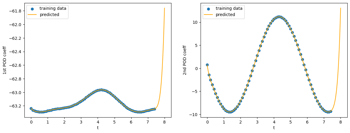
Figure 12. Plot between time and the predicted first two POD coefficients.

The predictive outcome based on the first 2 POD coefficients suggests that the PCE has not successfully captured the periodicity component from the POD coefficient despite of good fit in the training data region. Hence, a more appropriate model needs to be employed. However, I leave this task to the reader as an exercise.

Assuming that we have an appropriate model to predict the POD coefficient behaviour, now we predict the full flow field. Given that we already have the predicted POD coefficient, obtaining the full flow field can be easily done by:

In our case, let’s try to predict the flow field at $t=7.7 s$

def predict_all_coeff(x, pce_list):
    pred_coeffs = []
    x_norm = x/20  # normalize input with 20 (max t in dataset)
    for pce in pce_list:
        temp = pce(x_norm)
        pred_coeffs.append(temp)
    
    pred_coeffs = np.concatenate(pred_coeffs, axis=0)
    return pred_coeffs

pred_coeffs = predict_all_coeff(7.7, pce_list)
predicted_field = u_trunc @ pred_coeffs.reshape(-1,1)

# Try plotting first basis function of POD
ref = snapshot[:,77].reshape(50,100) # get first order basis
predicted = predicted_field[:,0].reshape(50,100) # get first order basis
fig1, ax1 = plt.subplots(1, 2, figsize=(14, 5))
# Plot full-order solution
cf = ax1[0].contourf(x_grid,y_grid,ref)
cbar = fig1.colorbar(cf, ax=ax1[0])
ax1[0].set_xlabel('X')
ax1[0].set_ylabel('Y')
ax1[0].set_title('Original field at t=7.7')
# Plot first basis function
cf1 = ax1[1].contourf(x_grid,y_grid,predicted)
cbar1 = fig1.colorbar(cf1, ax=ax1[1])
ax1[1].set_xlabel('X')
ax1[1].set_ylabel('Y')
ax1[1].set_title('Predicted field at t=7.7')
plt.show()

Figure 13. Predicted flow field at t=7.7 s.

Finally, we can conclude that proper orthogonal decomposition provides an effective way to reduce the dimensionality/complexity of the vector field problem into its lower dimension. However, to be able to accurately predict the behaviour of the system, a suitable prediction model needs to be chosen correctly. Nonetheless, this quick tutorial and overview provide a general idea of how to perform prediction on a complex vector field such as a flow field by reducing its dimensionality through proper orthogonal decomposition.

How to cite this article:

@misc{faza2024basicpodpce,
   author =       {Faza, Ghifari Adam},
   title =        {Simple Vector Field Prediction using Proper Orthogonal Decomposition and Polynomial Chaos Expansion (POD-PCE)},
   month =        {April},
   year =         {2024},
   url =          {https://fazaghifari.github.io/posts/2024/04/pod-pce-basic-en/},
 }

References

1. M. Loéve, Fonctions Al ́eatoires de Second Ordre (Random Functions of Second Order), Gauthier-Villars, 1970.
2. G. Berkooz, P. Holmes, J. L. Lumley, The proper orthogonal decomposition in the analysis of turbulent flows, Annual Review of Fluid Mechanics 25 (1993) 539–575. URL: https://doi.org/10.1146/annurev.fl.25.010193.002543. doi:10.1146/annurev.fl.25.010193.002543.
3. J. Cusumano, M. Sharkady, B. Kimble, Spatial coherence measurements of a chaotic flexible-beam impact oscillator (1993) aerospace structures: Nonlinear dynamics and system response, American Society of Mechanical Engineers, AD-33 (1993) 13–22.
4. A. Chatterjee, An introduction to the proper orthogonal decomposition, Current Science 78 (2000) 808–817. URL: http://www.jstor.org/stable/24103957.
5. https://en.wikipedia.org/wiki/Singular_value_decomposition#
6. R. Ghanem, P. D. Spanos, Polynomial chaos in stochastic finite elements, Journal of Applied Mechanics 57 (1990) 197–202. URL:https://doi.org/10.1115/1.2888303. doi:10.1115/1.2888303.
7. https://en.wikipedia.org/wiki/Legendre_polynomials
8. D. Xiu, G. E. Karniadakis, The wiener–askey polynomial chaos for stochastic differential equations, SIAM Journal on Scientific Computing 24 (2002) 619–644.URL: https://doi.org/10.1137/s1064827501387826.doi:10.1137/s1064827501387826